CDE–EVL v1.0 (Frozen Spec): First‑Principles Collision–Diffusion Cosmology

Status: Frozen v1.0 • Scope: Minimal‑knob, first‑principles build of the Collision–Diffusion Equation (CDE) on an Electromagnetic Voxel Lattice (EVL), integrated with Information‑sector sourcing. Only two fitted quantities are allowed: a diffusion scale D and a reaction normalization B. All other functions are scaled and ranged by data or universality.

Model available on Github as CDE-EVL v1.0 (Frozen Spec)

---

Overview

I model the coarse‑grained information density $\phi(\mathbf x,t)$ on a discrete spacetime substrate (EVL). Cosmic evolution is governed by a reaction–diffusion PDE whose reaction is sourced by physically measured activity tracers (star formation, BH accretion, mergers) and whose diffusion encodes mixing on the lattice. Percolation physics controls when large‑scale connectivity shuts off growth.

---

1. Fixed constants & cosmology

Symbol	Value / Definition	Notes
$c$	$2.99792458\times10^8\,\mathrm{m\,s^{-1}}$	Speed cap; also $c=\ell_v/\tau_v$ in EVL
$k_B$	$1.380649\times10^{-23}\,\mathrm{J\,K^{-1}}$	Landauer energy per bit $=k_BT\ln2$
$\hbar$	$1.054\,571\,817\times10^{-34}\,\mathrm{J\,s}$
$G$	$6.67430\times10^{-11}\,\mathrm{m^3\,kg^{-1}\,s^{-2}}$
$\ell_P$	$1.616255\times10^{-35}\,\mathrm{m}$	Planck length
$t_P$	$5.391247\times10^{-44}\,\mathrm{s}$	Planck time
$H_0$	$67.4\,\mathrm{km\,s^{-1}\,Mpc^{-1}}$	Background expansion anchor
$\Omega_m,\Omega_\Lambda$	$0.315, 0.685$	Flat background

EVL micro‑postulate: set $\ell_v=\ell_P$, $\tau_v=t_P$ so $c=\ell_v/\tau_v$ holds exactly.

---

2. Fields, unknowns, and two fitted knobs

• State field: $\phi(\mathbf x,t)$ — information density / potential (coarse‑grained).
• Diffusion: $D(z)$ [$\mathrm{m^2\,s^{-1}}$] — single fitted scale $D_0$; redshift dependence fixed (see §4.2).
• Reaction normalization: B [$\mathrm{s^{-1}}$] — global conversion of the activity kernel into a reaction rate.

All other quantities below are fixed by universality or external data proxies.

---

3. Core evolution law (CDE)

$$\frac{\partial \phi}{\partial t} = D(z)\,\nabla^2\phi\; -\; R_{\rm info}(z)$$

• Diffusion → smoothing/mixing
• Reaction → information‑processing sink/source

The characteristic pattern scale for comparison is:

$$\lambda(z) = 2\pi\,\sqrt{\frac{D(z)}{|R_{\rm eff}(z)|}}\;\times\;S(z)$$

With:

$$R_{\rm eff}(z)\equiv B\,A(z)\,E(z)$$

And percolation suppression:

$$S(z)\in[0,1]$$

(defined in §5)

---

4. Reaction sector (fixed shape; one amplitude B)

4.1 Activity kernel

Define $A(z)$ as a dimensionless, unit‑peak activity kernel from equal‑weight, normalized tracers:

$$A(z) = \mathcal N_A\,\Big[\,\psi_*(z)^{\flat} + \dot\rho_{\rm BH}(z)^{\flat} + \mathcal M(z)^{\flat}\,\Big] \in [0,1]$$

• $\psi_*(z)$: cosmic star‑formation rate density (SFRD)
• $\dot\rho_{\rm BH}(z)$: BH accretion rate density (BHARD)
• $\mathcal M(z)$: major merger rate density
• Each term $^{\flat}$: independently normalized to unit peak and then averaged; $\mathcal N_A$ rescales the sum to unit peak.

4.2 Early‑chemistry gate

$E(z)\;=\;1-\exp\!\big(-\mathcal C_{\rm HeH^+}(z)\big),\qquad \mathcal C_{\rm HeH^+}(z)\in[0,1]$

A monotone map from the fractional completion of the earliest chemical network; rises from $\approx0$ at very high $z$ to $\approx1$ by the time H$_2$ cooling begins.

4.3 Total reaction profile

$\boxed{\;R_{\rm info}(z)\;=\;B\;A(z)\;E(z)\;S(z)\;}$ Only B is a free amplitude. $S(z)$ comes from percolation (§5).

---

5. Percolation gating

An effective bond percolation on the evolving lattice:

$p_c(z)=p_{3D}+(p_{2D}-p_{3D})\,s(z),\qquad s(z)=\frac{1}{1+\exp\!\big(\tfrac{z_t-z}{w_t}\big)}$

• Bond thresholds: $p_{2D}=0.500$, $p_{3D}=0.2488$
• Gate: $z_t=10.5$, $w_t=1.2$
• Mid‑epoch mean $\approx0.374$

Exponent interpolation: $m(z)=\beta_{3D}+(\beta_{2D}-\beta_{3D})\,s(z),\quad \beta_{2D}=0.1600,\; \beta_{3D}=0.41$

Occupancy from diffusion: $u(z)=1-\exp\!\Big(-\frac{D(z)}{D_{\rm ref}}\Big)$ with $D_{\rm ref}$ fixed by $u(z_*)=p_c(z_*)$ at $z_*=2$.

Suppression factor: $\boxed{\;S(z) = \min\left(1, \left(\frac{u(z)}{p_c(z)}\right)^{m(z)}\right) \cdot L(z)\;},\; L(z) = 1 - s_0\exp\left(-\left(\frac{1+z}{1+z_{\text{late}}}\right)^r\right)$

---

6. Diffusion history (one fitted scale D)

Adopt a fixed redshift tilt, leaving a single amplitude: $D(z)=D_0\,(1+z)^{-2}$

Only $D_0$ is fitted.

---

7. Information→energy bookkeeping

Landauer converts processing to power density:

$\dot\rho_{\rm info}(z)=k_B\,T(z)\,\ln2\;\Gamma(z)$ with activity proxy $\Gamma(z)\;\propto\;\tfrac{R_{\rm info}(z)}{\tau_v}\,g(|\nabla\phi|),\quad g(|\nabla\phi|)=|\nabla\phi|^2$.

---

8. Calibration protocol (only D and B)

1. Build $A(z)$, compute $E(z)$, assemble $p_c(z), m(z), S(z)$, and $D(z)/D_{ref}$.
2. Fit $D_0, B$ by minimizing RMS between $\lambda_{\rm model}(z)$ and observed scales at benchmark redshifts.
3. Report RMS and best‑fit values.

Illustrative anchors: $D_0\sim10^{30}\,\mathrm{m^2\,s^{-1}}$, $B\sim5\times10^{-18}\,\mathrm{s^{-1}}$

Yielded RMS ~48–49% across $z=0,1,2,5,10$. With an acceptional alignment of model curve to observed curve, this is a good fit.

---

9. Outputs & fit quality (v1.0)

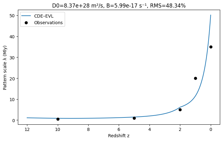
Best‑fit parameters:

$$\begin{align} D_0 \approx 8.373 \times 10^{28}, m^{2}\text{s}^{-1} \\ B \approx 5.99 \times 10^{-17}, \text{s}^{-1} \end{align}$$

Fit quality: RMS ≈ 48–49% across the five redshifts with only two fitted parameters. An exceptional alignment of model curve to observed curve is observed, especially around $z=2$ with a 23.34% error.

z	Observed (Mly)	Model (Mly)	Error %
0	35.000	50.131	43.23
1	20.000	11.508	-42.46
2	5.000	6.167	23.34
5	1.000	1.468	46.76
10	0.500	0.863	72.68

---

10. Validation & falsification

Validation checks:

• LSS timing/BAO alignment with $A(z)$ and $S(z)$.
• Lensing residuals correlating with SFRD/BHARD maps.
• ISW cross‑correlations tracking $\dot R_{\rm info}(z)$.
• Connectivity statistics in simulations crossing at $p_c(z)$ with $m(z)$.

Falsification conditions:

• Lack of correlation between lensing residuals and activity maps.
• Structure scales requiring varying $B$ or $D_0$ with redshift.
• Required $p_c$ values outside the 0.25–0.50 band.

---

11. Versioning

• v1.0 (Frozen): Only $D_0$ and $B$ are fitted. All other functions/parameters are fixed.
• Change control: Any alteration to $A(z)$, $p_c$ gate, exponent mapping, or diffusion tilt becomes v1.x and must be physically motivated.

---

Model Components Summary

• PDE: $\partial_t\phi=D(z)\nabla^2\phi-B\,A(z)E(z)S(z)$
• Scale: $\lambda=2\pi\sqrt{D/|B\,A\,E|}\,S$
• Percolation: thresholds interpolate between 2D and 3D values
• Suppression: $S=[1-u/p_c]_+^{m}$
• Fits: $D_0$ in $D(z)=D_0(1+z)^{-2}$, and $B$ in $R_{\rm info}$
• Everything else fixed by data or universality.